$$ \newcommand{\bx}{\boldsymbol{x}} \newcommand{\bt}{\boldsymbol{\theta}} \newcommand{\dkl}{\mathrm{d}_{\mathrm{KL}}} \newcommand{\dtv}{\mathrm{d}_{\mathrm{TV}}} \newcommand{\emv}{\hat{\theta}_{\mathrm{emv}}} \newcommand{\ent}{\mathrm{Ent}} $$

2  Lab work n°1

You can download the Lab Work n°1: Deep PDE Solver as a Jupyter Notebook file here. ¹

All the necessary informations are already included in the notebook². Below is a brief summary of the lab content and some expected results.

2.1 Summary of the lab

Content :

The Lab work is divided into 2 parts :

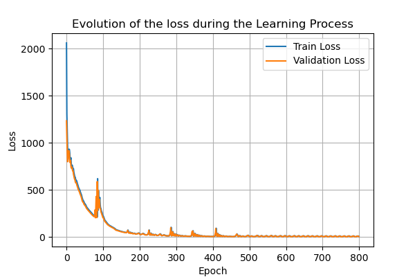
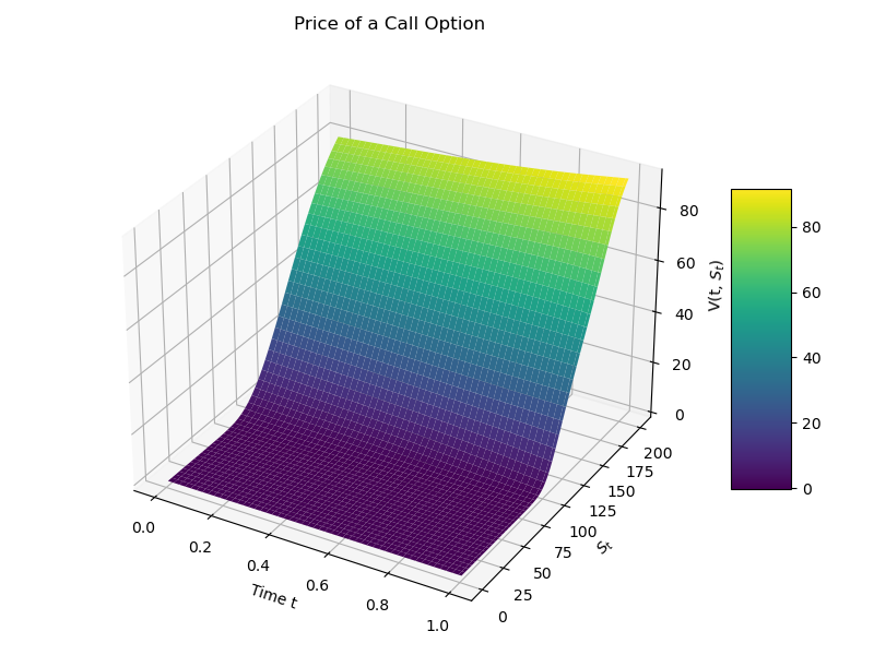
• The first part is devoted to the implementation of the Deep Galerkin algorithm where you are going to test it on various PDEs arising in finance. We give below some expected plots that you should obtain after finishing this part.

Evolution of the loss in the PDE learning of the call price

Price surface \((t,s) \mapsto C(t,s)\) for a call option

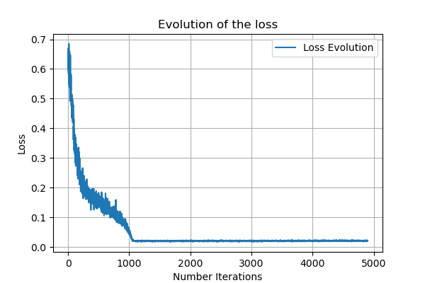
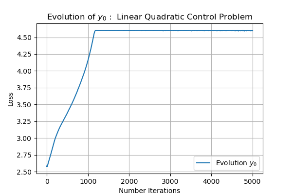
• The second part is devoted to the implementation of the Deep BSDE Solver where you are going to test it on known PDEs arising from finance and stochastic control problems. We give below some expected plots that you should obtain after finishing this part.

Evolution of the loss for \(y_0\) in the LQ control problem

Evolution of \(y_0\) in the LQ control problem

2.2 Towards the open ended project

The list of potential projects for the Deep Learning for PDE can be found in the PDF file by clicking here.

• Please do not forget to indicate your name on the Excel sheet here.
• Recall that the submission deadline for the mini-project and the answers to the lab session³ is set to 31 March 2026.

---

1. If you end-up with a .txt file, download it and rename it as a .ipynb file.

2. There will be coding and math questions.

3. No PDF submission is required for the lab session answers. The answers should be written directly in the Jupyter notebook and submitted along with the documents associated with the mini-project.